EOB Potential

import numpy as np; import matplotlib.pyplot as plt
import EOBRun_module 

def eob_potential(r, q, L=3.9):
    """
    Compute the EOB potential from the 5PNlog EOB A potential
    """
    nu          = q/(1+q)**2 
    A, dA, d2A  = EOBRun_module.eob_metric_A5PNlog_py(r, nu)
    return A*(1. + (L/r)**2)

def schw_potential(r, M=1,L=3.9):
    """
    Compute the Schwarschild potential
    """
    return (1 - 2*M/r)*(1 + (L/r)**2)

def hline_text(ax,x,y,txt, yb=1.001, color='k',linestyle='--',rotation=0):
    """
    Horizontal line with text
    """
    ax.axhline(y=y, color=color, linestyle=linestyle)
    ax.text(x,y*yb,txt, size=12) #,rotation=rotation)

def marker_text(ax,x,y,txt, yb=1.001,color='b',markersize=4,rotation=0):
    """
    Marker with text
    """
    ax.plot(x,y, 'o', color=color,
            markersize=markersize)
    ax.text(x,y*yb,txt)
    
def plot_teob_W():
    q     = 1
    pph   = 3.9
    E_hyp = 1.001

    r   = np.linspace(0.1,50,400)
    V_s = schw_potential(r, L=pph)
    V_e = np.array([eob_potential(ri, q, L=pph) for ri in r])
    iM  = np.argmax(V_e)
    im  = np.argmin(V_e[r>3]) + len(r[r<=3])

    # conservative plot
    ax = plt.subplot()
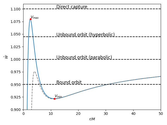
    ax.plot(r, V_e, label='Effective EOB potential')
    ax.plot(r, V_s, color='gray',linestyle='--', label='Effective Schw. potential')

    marker_text(ax,r[im],V_e[im],r'$V_{\rm min}$', color='r', yb=1.003)
    marker_text(ax,r[iM],V_e[iM],r'$V_{\rm max}$', color='r')

    hline_text(ax,12,0.95  , 'Bound orbit')
    hline_text(ax,12,1.00  , 'Unbound orbit (parabolic)')
    hline_text(ax,12,1.045 , 'Unbound orbit (hyperbolic)')
    hline_text(ax,12,1.1   , 'Direct capture')

    dummy, = plt.plot(0, 0, color='k', linestyle='--',label='Particle energy $E_0$')

    ax.set_ylim(0.9,1.11)
    ax.set_xlim(0,np.amax(r))
    ax.set_xlabel('$r / M $')
    ax.set_ylabel(r'$\hat{W}$')
    plt.tight_layout()
    plt.savefig('../template/assets/images/eobpot.png')
    plt.show()
    plt.close()

if __name__ == '__main__':
    plot_teob_W()