import numpy as np; import matplotlib.pyplot as plt
import EOBRun_module as EOB
import matplotlib.pyplot as plt
plt.rcParams["figure.figsize"] = (4,2)
# Use configurations from Tab. I of
# https://arxiv.org/pdf/2009.12857.pdf
data = {
# 1: {'rmin': None, 'E0': 1.0225555, 'p0': 4.3986080 },
2: {'rmin': 3.70, 'E0': 1.0225722, 'p0': 4.49039348 },
3: {'rmin': 4.03, 'E0': 1.0225791, 'p0': 4.58209352 },
4: {'rmin': 4.85, 'E0': 1.0225870, 'p0': 4.8570920 },
5: {'rmin': 5.34, 'E0': 1.0225870, 'p0': 5.0403920 },
6: {'rmin': 6.49, 'E0': 1.0225884, 'p0': 5.4986320 },
7: {'rmin': 7.59, 'E0': 1.0225924, 'p0': 5.9568680 },
8: {'rmin': 8.66, 'E0': 1.0225931, 'p0': 6.4150960 },
9: {'rmin': 9.72, 'E0': 1.0225938, 'p0': 6.8733240 },
10: {'rmin': 10.78,'E0': 1.0225932, 'p0': 7.33153432 }
}
def plot_chi():
chi = []
js = []
for k in data.keys():
jj = data[k]['p0']
pars = {
'M' : 1, # Total mass
'q' : 2, # Mass ratio m1/m2 > 1
'chi1' : 0., # Z component of chi_1
'chi2' : 0., # Z component of chi_2
'LambdaAl2' : 0., # Quadrupolar tidal parameter of body 1 (A)
'LambdaBl2' : 0., # Quadrupolar tidal parameter of body 2 (B)
'j_hyp' : jj, # Initial angular momentum
'H_hyp' : data[k]['E0'], # Initial energy
'r_hyp' : 100., # Initial separation
'domain' : 0, # Time domain. EOBSPA is not available for eccentric waveforms!
'srate_interp' : 4096., # srate at which to interpolate. Default = 4096.
'use_geometric_units': "yes", # output quantities in geometric units. Default = 1
'interp_uniform_grid': "yes", # interpolate mode by mode on a uniform grid. Default = 0 (no interpolation)
'use_mode_lm' : [1], # List of modes to use/output through EOBRunPy
'arg_out' : "yes", # Output hlm/hflm. Default = 0
}
t, _, hp, _, dyn = EOB.EOBRunPy(pars)
js.append(jj)
chi.append(dyn['phi'][-1] - dyn['phi'][0] - np.pi)
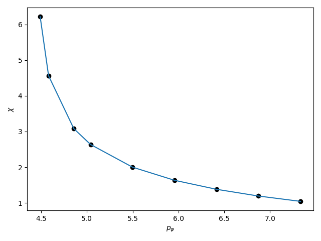
plt.plot(js, chi)
plt.scatter(js, chi, color='k')
plt.xlabel(r'$p_{\varphi}$')
plt.ylabel(r'$\chi$')
plt.tight_layout()
plt.show()
if __name__ == '__main__':
plot_chi()